Can do linear classification, nonlinear classification, linear regression, etc., compared to logical regression, linear regression, decision tree and other models (non-neural network)
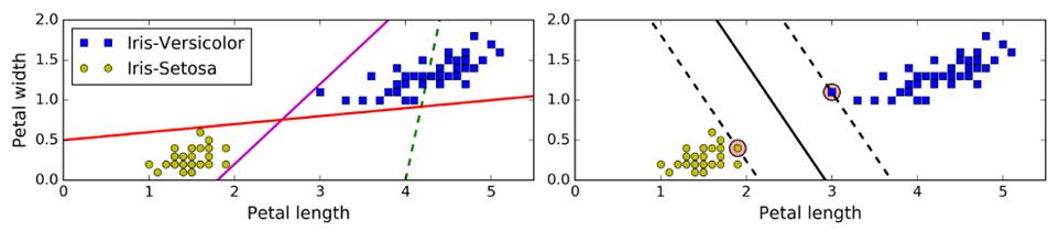
Traditional linear classification: select the centroid of two piles of data, and do the vertical line (low accuracy) - left
SVM: Fitting is not a line, but two parallel lines, and the width of these two parallel lines is as large as possible. The main focus is on the edge of the distance near the data point (support vector support vector), that is, large margin classification - above right
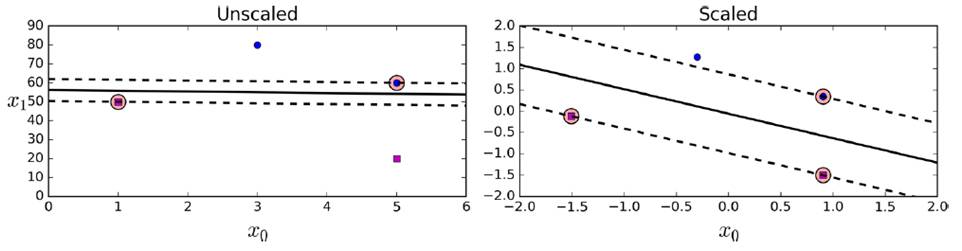
Before use, you need to do a scaling of the data set to make a better decision boundary.

But it is necessary to tolerate some points to cross the dividing boundary and improve the generalization, ie softmax classification
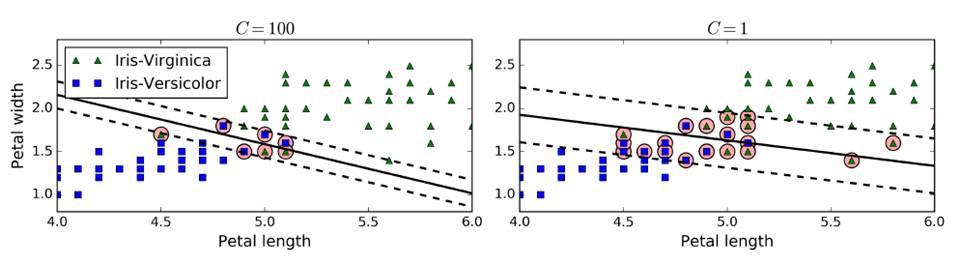
In sklearn, there is a hyperparameter c, which controls the complexity of the model. The larger c is, the smaller the tolerance is, the smaller c is, the higher the tolerance. c Add a new regular amount to control the SVM generalization ability to prevent overfitting. (Generally use gradsearch)
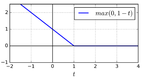
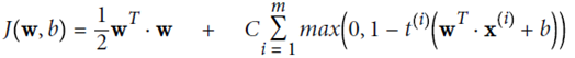
SVM-specific loss function Hinge Loss
(liblinear library, does not support kernel function, but relatively simple, complexity O (m * n))
Consistent with the characteristics of SVM, only consider vectors that fall near the classification surface and cross the classification surface to the other domain, giving a linear penalty (l1), or squared term (l2)
Import numpy as npfrom sklearn import datasetsfrom sklearn.pipeline import Pipelinefrom sklearn.preprocessing import StandardScalerfrom sklearn.svm import LinearSVCiris = datasets.load_iris()X = iris["data"][:,(2,3)]y = (iris[ "target"]==2).astype(np.float64)svm_clf = Pipeline(( ("scaler",StandardScaler()), ("Linear_svc",LinearSVC(C=1,loss="hinge")), ) )svm_clf.fit(X,y)print(svm_clf.predit([[5.5,1.7]]))
Classification of nonlinear data
There are two ways to construct high-dimensional features and construct similarity features.
Use high-dimensional spatial features (ie, the idea of ​​the kernel) to square the data, cubes. . Map to high dimensional space
From sklearn.preprocessing import PolynomialFeaturespolynomial_svm_clf = Pipeline(( ("poly_features", PolynomialFeatures(degree=3)), ("scaler", StandardScaler()), ("svm_clf", LinearSVC(C=10, loss="hinge") )))polynomial_svm_clf.fit(X, y)
This kind of kernel trick can greatly simplify the model, without the need to display the processing of high-dimensional features, you can calculate more complex situations.
But the more complex the model, the greater the risk of overfitting
SVC (based on the libsvm library, supports kernel functions, but relatively complex, can not use too large data, complexity O (m^2 * n) - O (m ^ 3 * n))
SVC can be used directly (coef0: high-order and low-order weights)
From sklearn.svm import SVCpoly_kernel_svm_clf = Pipeline(( ("scaler", StandardScaler()), ("svm_clf", SVC(kernel="poly", degree=3, coef0=1, C=5)) ))poly_kernel_svm_clf. Fit(X, y)
Add similarity features
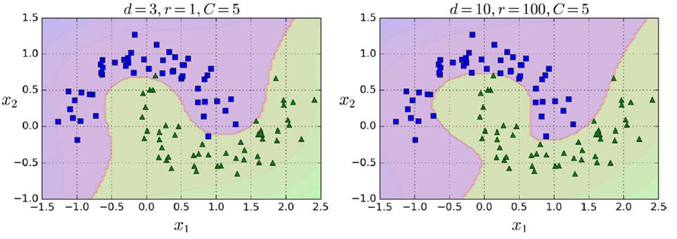
For example, the following figure creates a Gaussian distribution of x1 and x2, respectively, and then creates a new coordinate system to calculate the Gaussian distance (Gaussian RBF Kernel radial basis function).
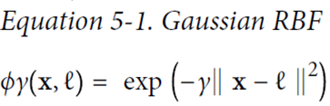
Gamma (γ) controls the shape of the Gaussian curve fat and thin, the distance between the data points plays a stronger role
Rbf_kernel_svm_clf = Pipeline(( ("scaler", StandardScaler()), ("svm_clf", SVC(kernel="rbf", gamma=5, C=0.001)) ))rbf_kernel_svm_clf.fit(X, y)
The following are the effects of different gamma and C values.
SGDClassifier (supports massive data, time complexity O(m*n))
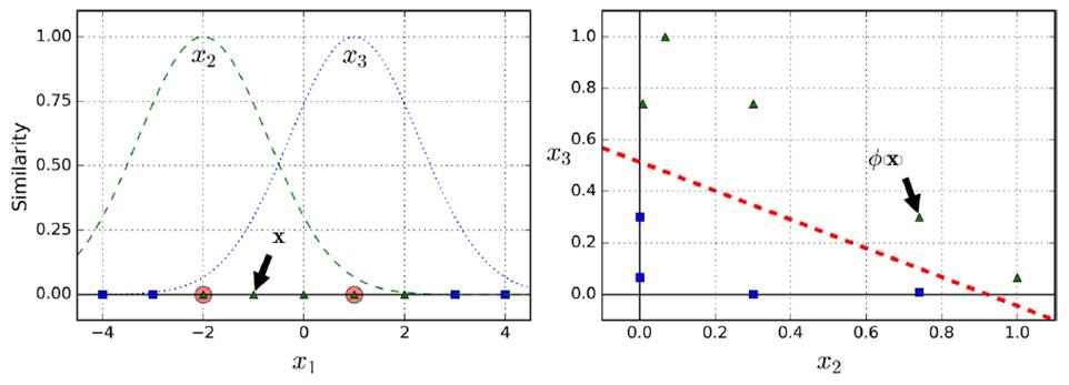
SVM Regression (SVM regression)
Try to make the used instance fit into the lane, and use the hyperparameter for the lane width.  Control, the bigger the wider the wider
Use LinearSVR
From sklearn.svm import LinearSVRsvm_reg = LinearSVR(epsilon=1.5)svm_reg.fit(X, y)
Using SVR
From sklearn.svm import SVRsvm_poly_reg = SVR(kernel="poly", degree=2, C=100, epsilon=0.1)svm_poly_reg.fit(X, y)
w control the width of the lane by controlling the angle of h tilt, the smaller the width, and the fewer data points that violate the classification
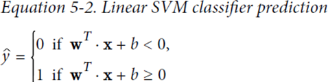
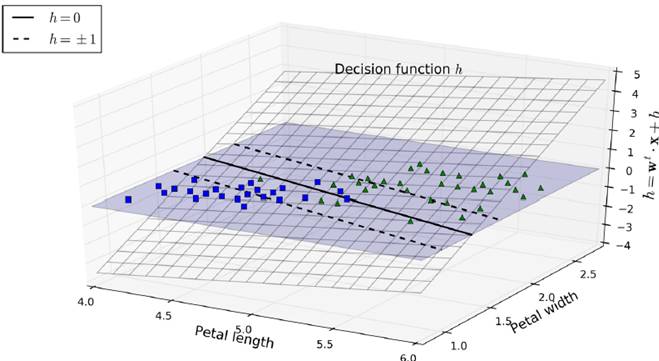
Hard margin linear SVM
optimize the target: 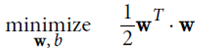 And guaranteed
Soft margin linear SVM
Add a new slack variable  Regularization
optimize the target: 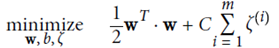 And guaranteed
Relaxation conditions, even if there are individual instances that violate the conditions, there is little punishment
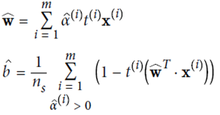
Calculated using the Lagrangian multiplier method, where α is the result of the relaxation term

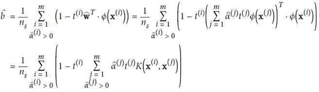
Calculation results:  take the average
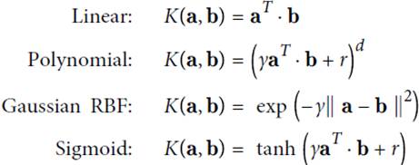
KernelizedSVM
due to 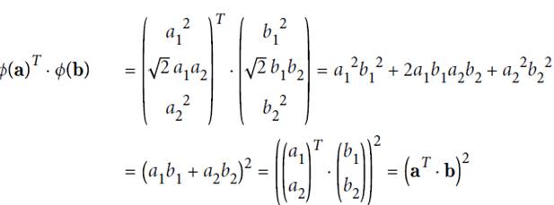
Therefore, the dot product calculation can be done first in the low space and then mapped into the high dimensional space.
The following formula indicates that the kernel trick can be calculated in high-dimensional space and calculated directly on low-dimensional dimensions.
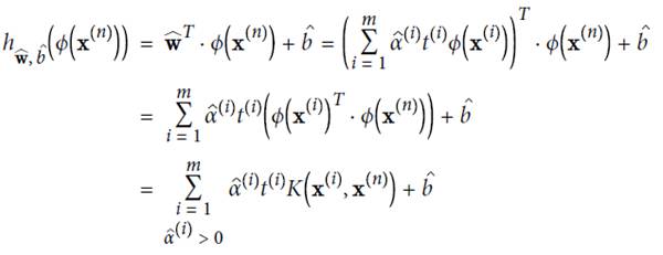
Several common kernals and their functions

About this item
- 9V Switching wall charger
- 110V input voltage / 9VDC 1A/2A/3A... output voltage
- For use with Arduino Uno, Mega and MB102 Power supply boards
- Connector size: 5.5 x 2.1mm/5.5*2.5mm...
- Center or Tip is positive, sleeve is negative
9v wall charger,AC Power Supply Wall Plug,Wall Adapter Power Supply,9V Power Adapter,ac 50/60hz power adapter,Wall Adapter Power Supply - 9VDC,100-240v converter switching power adapter
Shenzhen Waweis Technology Co., Ltd. , https://www.szwaweischarger.com