What is the status of Bayesian statistics in machine learning, and how is its principle and implementation process? This article introduces related concepts and principles.
Introduction : In the opinion of many analysts, Bayesian statistics are still difficult to understand. Due to the upsurge of machine learning , many of us have lost confidence in statistics. Our focus has been reduced to only exploring machine learning. Isn't it?
Is machine learning really the only way to solve real problems? In many cases, it does not help us to solve the problem, even if there are a lot of data in these issues. At the very least, you should know a certain amount of statistical knowledge. This will allow you to embark on complex data analysis problems regardless of the size of your data.
In the 1970s of the 18th century, Thomas Bayes proposed the "Bayesian theory," even after several centuries, Bayesian statistics have not diminished in importance. In fact, the best universities in the world are teaching in-depth courses on this topic.
Before truly introducing Bayesian statistics, first understand the concept of frequency statistics.
1. Frequency statistics
The debate over frequency statistics and Bayesian statistics has continued for several centuries, so it is important for beginners to understand the difference between the two and how to divide the two.
It is the most widely used inference technology in the field of statistics. In fact, it is the first school for beginners to enter the world of statistics. Frequency statistics detect whether an event (or hypothesis) has occurred. It calculates the probability of an event through long trials (tests are conducted under the same conditions).
Here, a fixed size sample distribution is used as an example. Then the experiment was theoretically infinitely repeated, but it actually had the intention of stopping. For example, when I have the intention of stopping in my mind, it repeats 1,000 times or I see at least 300 words in the coin flip process, I will stop experimenting. Let us now understand more:
We will understand the frequency statistics by flipping the coin. The purpose is to estimate the fairness of the tossed coin. The following table shows the number of times the toss is thrown:
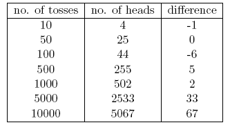
We know that the probability of getting a head on a fair coin flip is 0.5. We use No. of heads to indicate the actual number of heads on the head. Difference represents the difference between 0.5 (No. of tosses) and no. of heads .
It should be noted that although the number of throws increases, the difference between the actual number of heads and the expected number of heads (50% of the number of tosses) will gradually increase. But in terms of the total number of throws, the head appears to have a ratio of close to 0.5 (a fair coin).
In this experiment we found a very common defect in the frequency method: the independence of the experimental results and the number of experiments were duplicated.
2. Intrinsic defects in frequency statistics
Here, we begin to discuss the defects of frequency statistics:
In the 20th century, a large number of frequency statistics were applied to many models to detect whether the samples were different. It is important that one parameter be placed in various performances of the model and hypothesis tests. However, there are some major deficiencies in the design and implementation of frequency statistics. These problems in reality have attracted considerable attention. E.g:
1. p-values detect fixed-size samples. If two people work on the same data and have different braking intentions, they may get two different p-values .
2. The confidence interval (CI), like p-value , depends to a large extent on the size of the sample. Because no matter how many people perform the same data test, the results should be consistent.
3. Confidence intervals (CIs) are not probability distributions, so they do not provide the most likely values ​​and their parameters.
These three reasons are enough for you to think about the deficiencies of frequency statistics and why you need to consider the Bayesian approach.
The basic knowledge of Bayesian statistics is first understood here.
Bayesian statistics
“Bayesian statistics is a mathematical process that applies probabilities to statistical problems. It provides people tools to update the evidence in the data.†To better understand this problem, we need to understand some concepts. In addition, there are certain prerequisites:
Linear algebra
Probability Theory and Basic Statistics
3.1 Conditional probability
The conditional probability is defined as: the probability of a given event B in event A is equal to the probability that B and A occur together and is divided by the probability of B
For example: Set up two intersection sets A and B as shown in the figure below

Set A represents a set of events and set B represents another set. We want to calculate the probability that the probability of a given B has already occurred. Let's use red to represent the occurrence of event B.
Now, because B has already happened, the part of A that is important now is in the shade of blue. So, the probability of a given B is:

Therefore, the formula for event B is:
Either

Now, the second equation can be rewritten as:
This is the so-called conditional probability.
Assume that B is James Hunt's winning event and A is a raining event. therefore,
P(A) = 1/2, because every two days will be the next rain.
P(B) is 1/4 because James only wins once every four matches.
P(A | B) = 1, because James will win every time it rains.
Substituting a numerical value into the conditional probability formula gives us a probability of about 50%, which is almost twice that of 25% (it is not considered in the case of rain).
Perhaps, as you have guessed, it looks like Bayes' theorem .
Bayes' theorem is established at the top of the conditional probability and lies in the heart of Bayesian reasoning.
3.2 Bayes' Theorem
The following figure can help to understand the Bayesian theorem:
Now B can be written as
Therefore, the probability of B can be expressed as
but

So we get
This is the Bayesian theorem equation .
Bayesian reasoning
Let us understand the process behind Bayesian inference from the example of a coin flip:
An important part of Bayesian reasoning is the establishment of parameters and models.
Mathematical formulas for events observed by the model, parameters that affect the observed data in the model. For example, in the process of flipping a coin, the fairness of the coin can be defined as ?, which represents the parameter of the coin. The result of the event can be represented by D
The probability that the four coins are headed up is the fairness of a given coin (θ), ie P(D|θ)
Let us use Bayes' theorem to represent:
P(θ|D)=(P(D|θ) XP(θ))/P(D)
P(D|θ) is the possibility of our result given our given distribution θ. If we know that the coin is fair, this is the probability of observing the head up.
P(D) is evidence, because the probability of the data is determined by weighting the sum (or integration) of those specific values ​​that are θ at all possible values ​​of θ.
If the fairness of our coin is multiple views (but it is not known to be affirmative), then this tells us to see the probability that the certain order of flipping is all possibilities for our fair belief in the coin.
P(θ|D) is the observation, that is, our parameters after the number of heads.
4.1 Bernoulli approximation function
Looking back let us understand the likelihood function. So we learned that:
It is the probability of observing a specific number of heads that are flipped to a given number of coins for a given fairness. This means that our observation probability / ten thousand depends on the fairness of the coin (θ).
P(y=1|θ)=  [If the coin is fair θ = 0.5, the probability of observing the head (Y = 1) is 0.5]
P(y=0|θ)=  [If the coin is fair θ = 0.5, the probability of the tail is observed (Y = 0) is 0.5]
It is worth noting that 1 for the head and 0 for the tail is a model for the formulation of mathematical symbols. We can combine the above mathematical definitions into a single definition to represent the probabilities of the results of both.
P(Y |θ)= 
This is the so-called Bernoulli approximation function. The task of tossing coins is called the Bernoulli test.
y={0,1},θ=(0,1)
And, when we want to see a series of heads or flips, its probability is:
In addition, if we are interested in the probability of the number of heads being rolled up, the probability is as follows:
4.2 Pre-confidence distribution
This distribution is used to represent the distribution of our parameters based on past experience.
But what if one does not have previous experience?
Don't worry, mathematicians have come up with ways to alleviate this problem. It is considered as uninformative priors .
Then, used to represent the a priori mathematical function called beta distribution , it has some very beautiful mathematical characteristics, so that we have some understanding of the model about the binomial distribution.
Beta distribution of the probability density function is:

Here, our focus stays on the numerator, and the denominator is just to ensure that the integrated probability density function calculates to be 1.
α and β are called parameters of the shape-determining density function. Here, α is similar to the number of heads in the test, and β corresponds to the number of tails in the experiment. The following figure will help you visualize the distribution of α and β in different values
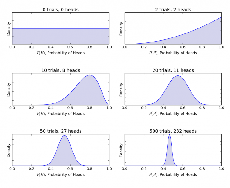
You can also draw your own Beta distribution using the code in R:
> library(stats)
> par(mfrow=c(3,2))
> x=seq(0,1,by=o.1)
> alpha=c(0,2,10,20,50,500)
> beta=c(0,2,8,11,27,232)
> for(i in 1:length(alpha)){
y<-dbeta(x,shape1=alpha[i],shape2=beta[i])
Plot(x,y,type="l")
}
Note: α and β are intuitive understandings, as they can be calculated from the known mean (μ) and the standard deviation of the distribution (σ). In fact, they are related:

If the distribution average and standard deviation are known, shape parameters can be easily calculated.
From the above chart you can infer:
When not throwing, we think that the fairness of coins can be depicted by a smooth line.
When the head appears more than the tail, the peak shown in the figure moves to the right side, indicating that the head is more likely to appear and the coins are unfair.
As more and more throwing operations are completed, the peak value of the larger proportion of heads narrows, which increases our confidence in the fairness of coin throwing.
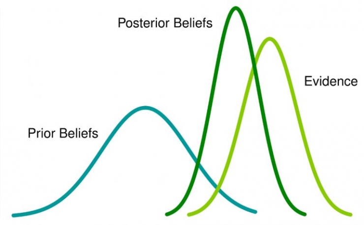
4.3 Post-confidence distribution
The reason we chose to believe before was to obtain a beta distribution, because when we multiply by an approximate function, the posterior distribution produces a form similar to the existing distribution, which is easy to relate and understand.
Calculate using Bayesian theorem


The formula between becomes
As long as you know the mean and our parameter criteria are published by θ , and by observing the head's N rollover, we can update our model parameter (θ) .
Let's use a simple example to understand this:
Assume that you think a coin is biased. It has a standard deviation of 0.1, an average (μ) deviation of about 0.6.
Then, α = 13.8, β = 9.2
Suppose you observe 80 heads up (z = 80 in 100 flips) (N = 100). then
Prior = P(θ|α,β)=P(θ|13.8,9.2)
Posterior = P(θ|z+α,N-z+β)=P(θ|93.8,29.2)
Image it:
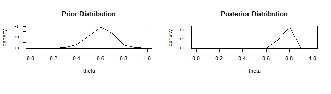
The above R code implementation process is:
> library(stats)
> x=seq(0,1,by=0.1)
> alpha=c(13.8,93.8)
> beta=c(9.2,29.2)
> for(i in 1:length(alpha)){
y<-dbeta(x,shape1=alpha[i],shape2=beta[i])
Plot(x,y,type="l",xlab = "theta",ylab = "density")
}
As more and more flips are performed and new data are observed, we can be further updated, which is the real power of Bayesian reasoning.
5. Test significance - frequency theory VS Bayes
Without using a strict mathematical structure, this section will provide different frequency theory and Bayesian method previews. A brief overview of the related, and which methods of the test group are most reliable, and their significance and diversity.
5.1 p-value
The distribution in the t-scores and fixed-size samples for a particular sample is calculated and then the p-value is also predicted. We can interpret the p-value as follows: (with a distribution of 0.02 with a mean value of 100): Samples with a 2% probability will have an average equal to 100.
This explanation shows that from the sampling of different size distributions, people are bound to get different values ​​of T, so the defects of different p values ​​are affected. A p-value less than 5% does not guarantee that the null hypothesis is wrong, nor does a p-value greater than 5% ensure that the null hypothesis is correct.
5.2 Confidence intervals
Confidence intervals have the same drawbacks, and because CI is not a probability distribution, there is no way to know which values ​​are most likely.
5.3 Bayesian factors
The Bayesian factor is the equivalent of the p-value in the Bayesian framework.
Zero-hypothesis in the Bayesian framework: only a certain value of one parameter (for example θ = 0.5) and zero probability assumed elsewhere ∞ probability distribution. (M1)
Another assumption is that all values ​​of θ are possible, so the representative distribution curve is flat. (M2)
The posterior distribution of new data is shown below.
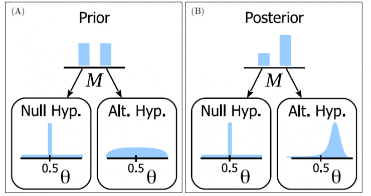
The various values ​​of θ represent Bayesian statistical adjustment confidence (probability). It can be easily seen that the probability distribution has turned to M2 with a higher value M1, ie M2 is more likely to occur.
The Bayesian factor does not depend on the actual distribution of θ but shifts between the amplitudes of M1 and M2.
In Panel A (above): The left column is the prior probability of the null hypothesis.
In Figure B (above), the left column is the posterior probability of the null hypothesis.
The Bayesian factor is defined as the comparison of the posterior probability with the existing one:

To reject the null hypothesis, BF <1/10 is preferred.
We can see the benefits of using Bayesian factors instead of p-values, which have independent intentions and sample sizes. Â
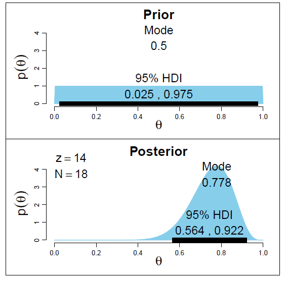
5.4 High Density Interval (HDI)
HDI is observed by the posterior distribution to observe the formation of new data. Since HDI is a probability, 95% of HDI gives the most reliable value of 95%. It also guarantees that 95% of the values ​​will be in different CI intervals.
Note that the first 95% of HDI is more extensive than the 95% posterior distribution because we added observations of new data in HDI.
Summary: Bayesian statistics, as a basic algorithm, occupies an important place in machine learning. Especially in data processing, it has a good classification effect on the probability of event occurrence and the reliability of the event.
PS : This article was compiled by Lei Feng Network (search "Lei Feng Network" public number attention) , refused to reprint without permission!
Via analyticsvidhya
This Automation curtain is specially designed for automation industry. SDKELI LSC2 light curtain is designed for automation field, with small size, compact structure and strong anti-interference ability, and the product meets IEC 61496-2 standards. The automatic light curtain is with reliable quality and very competitive price. It has been used in many factories and has replaced curtains from Omron, Banner, Keyence, etc.
Automatic Light Curtain,Laser Light Curtain,Automation Light Beam Sensor,Automatic Infrared Beam Sensor,Infrared Beam Curttain Sensor,Infrared Beam Sensor
Jining KeLi Photoelectronic Industrial Co.,Ltd , https://www.sdkelien.com